Mack's Stats

9.1. I revised this question, so please follow my description only. Conduct ANOVA (analysis of variance) and Regression coefficients to the data from cystfibr (> data (” cystfibr “) database. You can choose any variable you like. in your report, you need to state the result of Coefficients (intercept) to any variables you like both under ANOVA and multivariate analysis. I am specifically looking at your interpretation of R results. 

> library(ISwR)

> data(“cystfibr”)

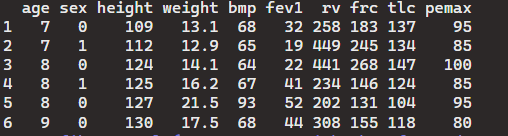
> head(cystfibr)

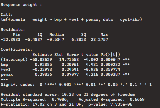
> cystfibrLM <- lm(pemax ~ age+weight+bmp+fev1, data = cystfibr)

> summary(cystfibrLM)

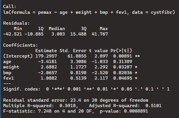
Because most p-values are less than the significant value of 0.5 the null hypothesis can be rejected(There is no correlation between the variables).

> anova(lm(pemax ~ age+weight+bmp+fev1, data = cystfibr))

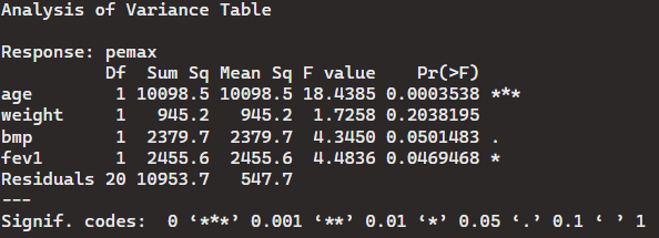
Again, here we can see that most of the p-values reject the null hypothesis. Although it looks like bmp may have a similar mean to pemax with this case of one DF (degree of freedom).

> mlm1 <- lm(cbind(age, weight) ~ bmp + fev1 + pemax, data = cystfibr)
> summary(mlm1)

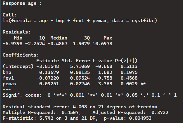
As you can see, calling a multivariate regression requires the use of the cbind function. The output shows two outcomes as if we called age and weight separately. Neither variables show any correlation between the other variables in the dataset. The standard error is much larger for age than it is weight which means if there is slight correlation, weight would have more than age.

9.2 The secher data (> data(“secher”) are best analyzed after log-transforming birth weight as well as the abdominal and biparietal diameters. Fit a prediction weight as well as abdominal and biparietal diameters. For a prediction equation for birth weight. How much is gained by using both diameters in a prediction equation? The sum of the two regression coefficients is almost identical and equal to 3.
Can this be given a nice interpretation to our analysis?
Please provide step by step on your analysis and code you use to find out the result. 

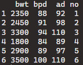
> data(“secher”)

> head(secher)

> Model10 <- lm((log(bwt))~ (I(log(ad))), data = secher)

> summary(Model10)

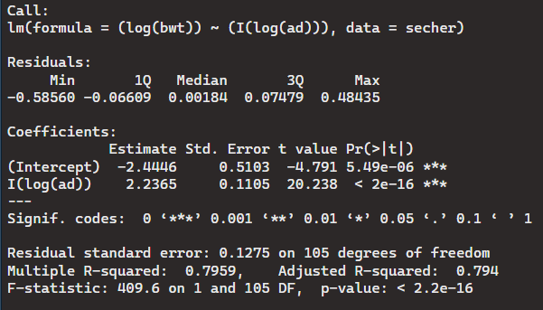
This accepts the alternative hypothesis that the variables are not associated. This is because the p-values are not at the significant value of 0.5.

> Model11 <- lm((log(bwt))~ (I(log(bpd))), data = secher)

> summary(Model11)

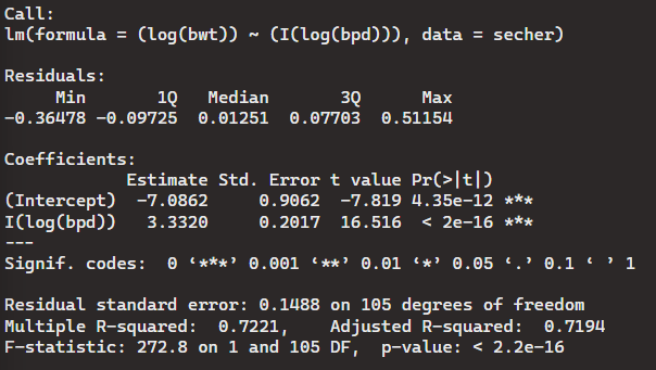
Again, in this case where the F-statistic is 272.8 on 1 and 105 degrees of freedom, and the p-value is < 2.2e-16, we accept the alternative hypothesis, and reject the null hypothesis.

> Model12 <- lm((log(bwt))~ (I(log(ad))) + (I(log(bpd))), data = secher)

> summary(Model12)

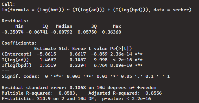
The sum of the two regression coefficients is almost identical and equal to 3. But, we still have to reject the null hypothesis in this case. Even though the variables of this dataset did not seem to have a correlation to each other, it was an interesting analysis to run. The r-squared values were always relatively close to 1 which shows a sign of some significance between the variables, but there was not enough proof to guarantee it.